A Fictional History of Numbers, Part 3: Computability, Reality, and Leaving Well Enough Alone.
Today we’re going to finish our discussion of the real numbers. We’ll see that they really are quite strange, in ways that are uncomfortable to think about, and then see why we keep using them anyway. And in passing we’ll define the computable numbers, which are an interesting type of number that doesn’t get nearly enough attention.
In part 1 we saw the most straightforward types of numbers, from the natural numbers that we count with, through the rationals that allow us to do basic arithmetic, to the algebraic numbers that let us solve polynomial equations. In part 2 we started asking questions about geometry, where we wanted to measure shapes. We found that the area of a circle isn’t given by an algebraic number, but can be approximated as closely as we want.
This led to the idea of completeness, which basically means that anything we can approximate has to be real. Every sequence that looks like it should converge does converge, and thus every length gets an actual number attached to it. And if we want completeness we get the real numbers, which can be thought of as the set of infinite decimals.
But the real numbers were hard to define. They seemed like a lot of work just to be able to talk about the area of a circle without making any estimates; ten decimal places should be enough for anybody, but the reals require infinitely many. In this essay we’ll see that it gets worse—but also that all that work really has a payoff, and that the real numbers are the right sort of numbers to use.
But first, if you want me to feel like my work has a payoff, please consider donating to my Ko-Fi account. Tips are never necessary, but always appreciated, and they help make it possible for me to keep writing essays like this one.
Reality is weird
We keep saying that the real numbers were really weird. How weird, exactly, are they?
We saw one hint with the observation that \(0.99\dots~ = 1 = 1.00\dots.\) All real numbers are infinite decimals, but sometimes more than one infinite decimal corresponds to the same real number. (And the idea that we can have “infinitely many nines”, and that somehow they add up to exactly one, is something that makes a lot of people viscerally uncomfortable). But that doubling-up is pretty easy to avoid if we’re careful; if we disallow decimal expansions that end in an infinite string of nines, the problem goes away, and we can sleep easy.
But the real numbers are strange in other ways. For instance: how many of them are there? There are two answers that both seem intuitively compelling. On the one hand, there are infinitely many real numbers, and maybe that’s all we can say. Infinity is infinity.
On the other hand, there are infinitely many natural numbers, and infinitely many rational numbers, and infinitely many real numbers. But it sure seems like there are more rational numbers than natural numbers, and more real numbers than natural numbers; so maybe all infinities aren’t the same.
If we look at this more carefully, things get complicated.
Even counting
How can we tell if two sets of things are the same size? We could try counting them and comparing the numbers: I have two hands, and two feet, so I have the same amount of hands and feet. But that doesn’t work if we have infinities. And anyway, counting is pretty abstract. Can we make things simpler?
There are a few approaches you could take here, but one very basic idea is just to pair things off. I don’t actually know how many pairs of shoes I have; but I know that I have the same number of left shoes and right shoes, because each left shoe is paired to a right shoe, and each right shoe is paired to a left shoe. There are none left over, so I have the same number of each. In technical terms, we’d say this table gives a bijection or a one-to-one correspondence between my left shoes and my right shoes.
On the other hand, if I try to pair up my socks and my shoes, I’ll have socks left over. I can give each shoe its own sock, and I’ll still have a big pile of socks left over. So I know I have more socks than shoes.
Let’s apply that idea now. Are there more natural numbers, or more even numbers? The obvious answer is that there are more natural numbers. If we look at the first ten numbers, only five of them are even.
| Natural numbers: | 1 | 2 | 3 | 4 | 5 | 6 | 7 | 8 | 9 | 10 | \(\dots\) |
| Even numbers: | 2 | 4 | 6 | 8 | 10 | \(\dots\) |
When we look at the first ten numbers, we have a lot of leftover (odd) natural numbers after we’ve paired off all the evens. And this pattern continues: if we look at the first hundred numbers, fifty of them are even. If we look at the first \(n\) numbers, about half of them will be even. So it seems like there must be more natural numbers than even numbers.
On the other hand, we can make a table like this, instead:
| Natural numbers: | 1 | 2 | 3 | 4 | 5 | 6 | 7 | 8 | 9 | 10 | \(\dots\) |
| Even numbers: | 2 | 4 | 6 | 8 | 10 | 12 | 14 | 16 | 18 | 20 | \( \dots \) |
In this table, every even number corresponds to a natural number, and every natural number corresponds to an even number. They’re perfectly paired up. So by this argument, there must be the same number of natural numbers and even numbers.
This is one of the weird things that immediately happens when we start dealing with infinities: an infinite set can be in bijection with one of its own subsets. We see this in the observation that “infinity plus one” is just infinity, since adding an element to an infinite set doesn’t change the size. And these bijections are surprisingly common; sets in bijection with the natural numbes include the perfect squares:
| Natural numbers: | 1 | 2 | 3 | 4 | 5 | 6 | 7 | 8 | 9 | 10 | \(\dots\) |
| Squares: | 1 | 4 | 9 | 16 | 25 | 36 | 49 | 64 | 81 | 100 | \( \dots \) |
the primes:
| Natural numbers: | 1 | 2 | 3 | 4 | 5 | 6 | 7 | 8 | 9 | 10 | \(\dots\) |
| Primes: | 2 | 3 | 5 | 7 | 11 | 13 | 17 | 19 | 23 | 29 | \( \dots \) |
and even the integers:
| Natural numbers: | 1 | 2 | 3 | 4 | 5 | 6 | 7 | 8 | 9 | 10 | \(\dots\) |
| Integers: | 0 | 1 | -1 | 2 | -2 | 3 | -3 | 4 | -4 | 5 | \( \dots \) |
We call these sets countable or countably infinite, because we can put all the elements in order and count them. It makes sense to ask for the \(37\)th prime number \((157),\) or the \(53\)rd square \((2809).\) And conversely, we can look at \(193\) and determine it’s the \(44\)th prime number, or at \(289\) and see it’s the \(17\)th square.
Counting the rationals
Let’s make things a little more interesting. We saw that the sets of natural numbers, integers, even numbers, perfect squares, and prime numbers were all the same size. What about the rational numbers? It seems like there are a lot more rational numbers than there are natural numbers. But it seemed like there were a lot more natural numbers than even numbers, and that didn’t work out, so we should look closer. We can try making a table like this:
| Natural numbers: | 1 | 2 | 3 | 4 | 5 | 6 | 7 | 8 | 9 | 10 | \(\dots\) |
| Rational numbers: | 1/1 | 1/2 | 1/3 | 1/4 | 1/5 | 1/6 | 1/7 | 1/8 | 1/9 | 1/10 | \( \dots \) |
But that won’t get us very far. Or rather, it would get us really far—we could keep going forever—but we’d leave most of the rational numbers out. We’ll never get to \(2\) that way.
Georg Cantor’s clever idea was to put the rational numbers on a grid, instead.
| 1/1 | 1/2 | 1/3 | 1/4 | 1/5 | 1/6 | 1/7 | 1/8 | 1/9 | … |
| 2/1 | 2/2 | 2/3 | 2/4 | 2/5 | 2/6 | 2/7 | 2/8 | 2/9 | … |
| 3/1 | 3/2 | 3/3 | 3/4 | 3/5 | 3/6 | 3/7 | 3/8 | 3/9 | … |
| 4/1 | 4/2 | 4/3 | 4/4 | 4/5 | 4/6 | 4/7 | 4/8 | 4/9 | … |
| 5/1 | 5/2 | 5/3 | 5/4 | 5/5 | 5/6 | 5/7 | 5/8 | 5/9 | … |
| 6/1 | 6/2 | 6/3 | 6/4 | 6/5 | 6/6 | 6/7 | 6/8 | 6/9 | … |
| 7/1 | 7/2 | 7/3 | 7/4 | 7/5 | 7/6 | 7/7 | 7/8 | 7/9 | … |
| 8/1 | 8/2 | 8/3 | 8/4 | 8/5 | 8/6 | 8/7 | 8/8 | 8/9 | … |
| 9/1 | 9/2 | 9/3 | 9/4 | 9/5 | 9/6 | 9/7 | 9/8 | 9/9 | … |
| ⋮ | ⋮ | ⋮ | ⋮ | ⋮ | ⋮ | ⋮ | ⋮ | ⋮ | ⋱ |
A grid like this should contain every positive1 rational number somewhere. In fact, the big problem is that some of them show up more than once! \(1/1 = 2/2 = 3/3\) and \(1/2 = 2/4 = 4/8\); we get a lot of repetitions. If we throw out the duplicates, and only include fractions that are in lowest terms, we get this:
| 1/1 | 1/2 | 1/3 | 1/4 | 1/5 | 1/6 | 1/7 | 1/8 | 1/9 | … |
| 2/1 | 2/3 | 2/5 | 2/7 | 2/9 | … | ||||
| 3/1 | 3/2 | 3/4 | 3/5 | 3/7 | 3/8 | … | |||
| 4/1 | 4/3 | 4/5 | 4/7 | 4/9 | … | ||||
| 5/1 | 5/2 | 5/3 | 5/4 | 5/6 | 5/7 | 5/8 | 5/9 | … | |
| 6/1 | 6/5 | 6/7 | … | ||||||
| 7/1 | 7/2 | 7/3 | 7/4 | 7/5 | 7/6 | 7/8 | 7/9 | … | |
| 8/1 | 8/3 | 8/5 | 8/7 | 8/9 | … | ||||
| 9/1 | 9/2 | 9/4 | 9/5 | 9/7 | 9/8 | … | |||
| ⋮ | ⋮ | ⋮ | ⋮ | ⋮ | ⋮ | ⋮ | ⋮ | ⋮ | ⋱ |
And once we have all the rational numbers in a grid like this, we can put them in order: we just have to take a snaking diagonal path through our grid.
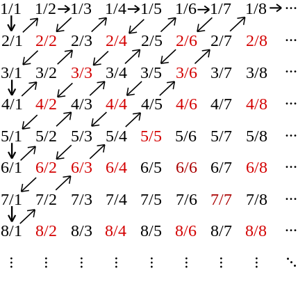
You can think of this as listing all the numbers where the top plus the bottom is two, then all the numbers where it’s three, then all the numbers where it’s four; there’s only a finite collection at each level.2 And that means that any rational number gets a specific, finite place in our list: \[ 1/1, \quad 2/1, \quad 1/2, \quad 1/3, \quad 3/1, \quad 4/1, \quad 3/2, \quad 2/3, \quad 1/4, \quad 1/5, \quad \dots \]
But all this is still a little weird, right? There are “obviously” way more rational numbers than there are natural numbers, but we just put them in order and paired them up. The fifth rational number is \(3\), and \(2/3\) is the eighth rational number; we can go in either direction.
Counting the algebraic numbers
We can take this logic one step further. In part 1 we defined the algebraic numbers, the numbers that are solutions to polynomial equations with integer3 coefficients. These include all the rational numbers, and all the square roots, and the imaginary number \(i\), and the solutions to \(x^5+x+3=0\) which we can’t describe any better than that. Can we pair them up with the rational numbers?
It seems obvious that there are way more algebraic numbers than rational numbers. But it was also “obvious” that there were more rational numbers than integers, and that didn’t quite pan out. In fact we can count the algebraic numbers. Take a minute and see if you can figure out how to do it!
There are a few approaches, but I think the easiest is this. First think about all the degree-one polynomials whose coefficients are \(1\) or smaller. There aren’t very many of these, and we can list them all off:
\[ \begin{aligned} 0 && 1 && -1 \\ x && x+1 && x-1 \\ -x && -x+1 && -x-1 \end{aligned} \] There are nine of them, so we can put them in whatever order we want. And each one has at most one root, so we’ve counted up to nine algebraic numbers. (In fact we’ve only counted three, since there’s a lot of duplication here, but that’s fine; we’ll just cross out the duplicate numbers like we did for the rationals.)
Now think about all the degree-two polynomials whose coefficients are \(2\) or smaller. There are a lot more of these!
Click to see all 125 degree-two polynomials whose coefficients are \\(2\\) or smaller.
\[ \begin{aligned} -2 && -1 && 0 && 1 && 2 \\ x-2 && x-1 && x && x+1 && x+2 \\ 2x-2 && 2x-1 && 2x && 2x+1 && 2x+2 \\ -x-2 && -x-1 && -x && -x+1 && -x+2 \\ -2x-2 && -2x-1 && -2x && -2x+1 && -2x+2 \\ x^2-2 && x^2-1 && x^2 && x^2+1 && x^2+2 \\ x^2+x-2 && x^2+x-1 && x^2+x && x^2+x+1 && x^2+x+2 \\ x^2+2x-2 && x^2+2x-1 && x^2+2x && x^2+2x+1 && x^2+2x+2 \\ x^2-x-2 && x^2-x-1 && x^2-x && x^2-x+1 && x^2-x+2 \\ x^2-2x-2 && x^2-2x-1 && x^2-2x && x^2-2x+1 && x^2-2x+2 \\ 2x^2-2 && 2x^2-1 && 2x^2 && 2x^2+1 && 2x^2+2 \\ 2x^2+x-2 && 2x^2+x-1 && 2x^2+x && 2x^2+x+1 && 2x^2+x+2 \\ 2x^2+2x-2 && 2x^2+2x-1 && 2x^2+2x && 2x^2+2x+1 && 2x^2+2x+2 \\ 2x^2-x-2 && 2x^2-x-1 && 2x^2-x && 2x^2-x+1 && 2x^2-x+2 \\ 2x^2-2x-2 && 2x^2-2x-1 && 2x^2-2x && 2x^2-2x+1 && 2x^2-2x+2 \\ -x^2-2 && -x^2-1 && -x^2 && -x^2+1 && -x^2+2 \\ -x^2+x-2 && -x^2+x-1 && -x^2+x && -x^2+x+1 && -x^2+x+2 \\ -x^2+2x-2 && -x^2+2x-1 && -x^2+2x && -x^2+2x+1 && -x^2+2x+2 \\ -x^2-x-2 && -x^2-x-1 && -x^2-x && -x^2-x+1 && -x^2-x+2 \\ -x^2-2x-2 && -x^2-2x-1 && -x^2-2x && -x^2-2x+1 && -x^2-2x+2 \\ -2x^2-2 && -2x^2-1 && -2x^2 && -2x^2+1 && -2x^2+2 \\ -2x^2+x-2 && -2x^2+x-1 && -2x^2+x && -2x^2+x+1 && -2x^2+x+2 \\ -2x^2+2x-2 && -2x^2+2x-1 && -2x^2+2x && -2x^2+2x+1 && -2x^2+2x+2 \\ -2x^2-x-2 && -2x^2-x-1 && -2x^2-x && -2x^2-x+1 && -2x^2-x+2 \\ -2x^2-2x-2 && -2x^2-2x-1 && -2x^2-2x && -2x^2-2x+1 && -2x^2-2x+2 \\ \end{aligned} \]
But it’s still a finite list, and each one has at most two solutions. So this has less than \(250\) algebraic numbers on it, and we can count them. In fact, let’s put the ones from the first list first, and then all the rest.
And now what we’ve done is defined a “height” for our polynomials: it’s the maximum of the degree and all the coefficients. So next week can look at the “height three” polynomials, the degree-three polynomials with coefficients three or less; and then the height four polynomials, which are degree-four polynomials with coefficients four or less; and so on.
At each height we’re adding finitely many algebraic numbers, so we can put them all in order. But we’ll get to every algebraic number eventually. For instance, the polynomial \(x^5+x+3\) has height five, so all the solutions will show up at the fifth step of this process. And that means we can pair the algebraic numbers up with the natural numbers. The algebraic numbers are countable.
Reality is too big
Counting the Reals
At this point you might be wondering if we can just always do this. The naturals and the rationals and the algebraics are all the same size; maybe infinities are all the same, after all. But let’s look at one more example: the real numbers.
Imagine we can put all the real numbers in a list, like we did for the rational numbers. Every real number can be written as an infinite decimal, so the list might look something like this:
\[ \begin{aligned} 7.77000643096\dots \\ 1.05898980495\dots \\ 6.35097622647\dots \\ 1.79660844929\dots \\ 4.45063253213\dots \\ 7.48984022493\dots \\ 2.23729615260\dots \\ 0.09015630234\dots \\ 1.30480398871\dots \\ 7.76421175135\dots \\ \end{aligned} \]
But now we can make a new infinite decimal, that definitely isn’t on the list. To keep things simple, we’ll make a number whose whole number part, to the left of the decimal point, is just \(0\). That means our number will be between \(0\) and \(1\), and that’s fine.
Now let’s look back at the big list. The first number on the list has a \(7\) in the first decimal place. So to make sure our number is different, the first decimal place can’t have a \(7\), so we’ll put a \(0\) there instead.
Now the second number on the list has a \(5\) in the second decimal place. To make sure our number is different, the second decimal place can’t have a \(5\), so we’ll put a \(0\) there instead.
The third number has a \(0\) in the third decimal place, so we don’t want to have a \(0\) in the third decimal place of our number; let’s use a \(1\) instead. At this point, we know the first three places of our infinite decimal: \(0.001\dots.\) And we also know that our infinite decimal isn’t any of the first three numbers on the big list.
So we can continue this pattern. The fourth digit of the fourth number is \(6\), so we can pick \(0\) for our fourth digit.4 The fifth digit of the fifth number is \(3\), so we can pick \(0\). The sixth digit of the sixth number is \(0\), so we have to pick something else like \(1\). The seventh digit of the seventh number is \(1\), and the eighth digit of the eighth number is \(0\), so we should pick \(0\) for our seventh digit and \(1\) for our eighth digit. As we keep going, we get the number
\[ 0.0010010100\dots \] which can’t5 be the same as any of the numbers on our list: \[ \begin{aligned} 7.\color{red}{7}7000643096\dots \\ 1.0\color{red}{5}898980495\dots \\ 6.35\color{red}{0}97622647\dots \\ 1.796\color{red}{6}0844929\dots \\ 4.4506\color{red}{3}253213\dots \\ 7.48984\color{red}{0}22493\dots \\ 2.237296\color{red}{1}5260\dots \\ 0.0901563\color{red}{0}234\dots \\ 1.30480398\color{red}{8}71\dots \\ 7.764211751\color{red}{3}5\dots \\ \end{aligned} \]
And that means that we have a number that isn’t on the infinite list we started with.
Now obviously we could make a list that contains this number. We can just tack it on to the front:6
\[ \begin{aligned} &0.0010010100\dots \\ &7.77000643096\dots \\ &1.05898980495\dots \\ &6.35097622647\dots \\ &1.79660844929\dots \\ &4.45063253213\dots \\ &7.48984022493\dots \\ &2.23729615260\dots \\ &0.09015630234\dots \\ &1.30480398871\dots \\ &7.76421175135\dots \\ \end{aligned} \]
And this list does have the number we just made. But it still can’t have every number on it; we can do the same thing we just did to get a new number, \(0.1000100000\dots,\) that isn’t on this list. Whatever list we come up with, there has to be a number that isn’t on it.
And in fact there are infinitely many numbers that aren’t on the list! We can see this pretty directly by listing a bunch of them. We built a number that wasn’t on the list, using just the digits \(0\) and \(1.\) But we could also use \(0\) and \(2,\) or \(4\) and \(7,\) or whichever pair of numbers we want. We could even choose a different pair for each place; we wind up having nine choices for each decimal place. So we can see all the following numbers aren’t on our original list:
\[ \begin{aligned} 0.0020020200 \dots \\ 0.4777777777 \dots \\ 0.6669666666 \dots \\ 0.1234567890 \dots \end{aligned} \]
And every number on that super-infinite is between \(0\) and \(1.\) We can find another infinite list between \(1\) and \(2,\) and another between \(2\) and \(3,\) and another between \(37\) and \(38.\) So not only are there more real numbers than natural, rational, or algebraic numbers; there are way, way more of them.
Leaving things up to chance
Another way of thinking about how many real numbers there are is to imagine choosing one at random. In fact, let’s just choose a number between \(0\) and \(1.\) Some of the numbers between \(0\) and \(1\) are rational, and others are irrational. So what are the odds that our randomly chosen number will be rational?
It turns out this probability of getting a rational number has to be zero. Not just small, but actually zero—even though it’s obviously possible, it has to be infinitely unlikely.
To see why, imagine that there was some positive probability of getting a rational number, like one in three.7 That would mean that one third of all the real numbers were rational—and that means we could divide the real numbers up into three sets \(A, B, C\), each of which are the size of the rational numbers.
But we know the rationals are countable, meaning we can put them in a numbered list. If the other two sets are the same size, we must be able to put them in lists, too, so we could divide the real numbers into three countable sets. And then we can make a complete list of all the real numbers: we can take the first element of \(A\), then the first element of \(B\), then the first element of \(C;\) then the second elements of \(A\) and \(B\) and \(C\); then the third elements; and so on. But this can’t possibly work, because we know the real numbers are uncountable. The rationals can’t be one third of the reals.
And the specific number was irrelevant here, right? If the rationals were \(1/1,000,000\) of the reals, we could still count the reals. We’d take the first element from each of our million sets, and then the second element, and then the third… If the rationals were any finite percentage of the real numbers, we’d be able to make a list of all the reals. So instead the rationals have to be zero percent of the real numbers.
And this sort of weirdness can only happen with infinities. Obviously there are rational numbers. “One” is a rational number, and it definitely exists. So if you pick a real number, it is possible to pick a rational number. But it will happen zero percent of the time. Not a small percentage; not a tiny percentage; it will happen zero percent of the time. There are infinitely many more real numbers than rational numbers. And that’s weird!
It gets worse when you realize the same argument applies to the algebraic numbers. It’s hard to come up with a real number that isn’t algebraic. Sure there are a couple of weird ones like \(\pi\) and \(e,\) but for the most part the irrational numbers we think about are all algebraic.
And yet if you pick a real number at random, there’s a zero percent chance you’ll get anything algebraic. There are infinitely more real numbers that aren’t solutions to polynomial equations than ones that are. Most real numbers are a little hard to even describe.
What are we even talking about?
And this brings us to weird you might have noticed when we showed that the reals were uncountable. We started with a list of real numbers, and we constructed a decimal that wasn’t on that list, and said we came up with \(0.0010010100 \dots. \) But did we really find a specific numbers? I wrote an ellipsis there; do we know what comes next?
And the answer is, sort of. We have a rule that tells us how to choose the next digit, so in theory we should know what comes next. But the rule depends on the next number on the original list, and I didn’t tell you that, so we can’t actually figure out the next digit.
In general we’ve been pretty sloppy about this! I said a real number is an infinite decimal, and I’ve been writing strings of digits with ellipses at the end to say the decimal keeps going. But consider these three real numbers:
\[ \begin{aligned} A & = 0.1428571428 \dots \\ B & = 3.1415926535 \dots \\ C & = 0.9193470019 \dots \end{aligned} \]
Do we know what digit comes next in \(A\)? It looks like it’s repeating, so we can guess the next digits are \(5\) and \(7\). (We might even notice this is the decimal expansion of \(1/7\), which can make us more confident in our guess.) For \(B\), we might recognize that this is \(\pi,\) so we can look up the next digits, which are \(8\) and \(9\). But what about for \(C\)? Can you figure out what comes next?
And in this case, you can’t. You absolutely can’t. I just generated ten random numbers, without any pattern, and wrote them down. I wrote an ellipsis like there’s something that comes next, but I never decided what comes next, so the ellipsis is basically a lie. I have no idea what that number is—except that it’s between \(\dfrac{9193470019}{10000000000} \) and \(\dfrac{9193470020}{10000000000}.\)
And honestly, that’s enough information to do pretty much any calculation we would actually want to do in the real world. But it’s not enough to tell you which specific real number this is. There are infinitely many—uncountably many!—ways to continue on from those ten digits and get a real number. And even I can’t really tell you which one I want.
Working with recipes
But I did tell you exactly what numbers \(A\) and \(B\) were—just not by writing down an infinite decimal. \(A\) is a repeating decimal, so I can give you a few digits and then tell you it repeats. \(B\) isn’t repeating, but it is a special number, \(\pi,\) and you can go look up the next digits if you want to. So rather than listing off all of the infinitely many digits, I can give you an algorithm, or recipe, for finding the digits. And you can keep computing the next digit and the next, for as long as you want. If a number has a recipe like this, that lets you compute all of the digits, we say it’s computable.
Can we do something like that for \(C?\) Can we take any infinite decimal and give an algorithm that will compute it?
Unfortunately, the answer is no, and for the same basic reason we know most real numbers aren’t algebraic. Every computable number has to have a recipe, so let’s think about what a recipe should look like. First, the recipe should be finite. We might not be able to finish reading the infinite decimal, but we should be able to finish reading the recipe. (Otherwise the recipe could just be a list of all the digits, which is missing the point!)
And we have to pick some language to write the recipe in. What language we pick doesn’t really matter; we could use English, or Mandarin, or some sort of weird mathematical symbology. But the language probably has finitely many symbols in it. Even if it has infinitely many symbols, we can limit it to a countable infinity—no more symbols than there are natural numbers.8
And with just those two restrictions, we find that we can count all the recipes. We can count the symbols, meaning we can label them so that there’s a first symbol, then a second, then a third, and so on. There’s at most one recipe that uses only the first symbol, and is only one symbol long. There are at most six recipes that use the first two symbols and are only two symbols long. There are at most \(39\) recipes that use the first three symbols and are only three symbols long.
We’ve found a height for our recipes again: the maximum of the length of the recipe, and the number of symbols off our list we have to use. There are finitely many recipes of each height, so we can label all the height-one recipes, then all the height-two recipes, then the height-three, then the height-four, and so on. Eventually we will reach every possible recipe, which means we can make a numbered list of every possible recipe.
This means the recipes are countable, and so the numbers they produce are also countable. So there are countably many computable numbers, but uncountably many real numbers. And just like with the rational numbers and the algebraic numbers, almost every real number is uncomputable; if we pick a random real number, it is essentially guaranteed not to be computable.
And to be clear about what this means: one hundred percent of the real numbers are things that we can’t even describe. They’re so strange and gratuitously infinite that we can’t even really talk about most of them.
So what are they good for?
The real numbers were hard to define. (It took basically all of part 2!) There are way too many of them, and almost all of them can’t even be described in a useful way. And if you think about them too hard, they just start seeming really weird and uncomfortable. So why do we keep using them, rather than doing something more sensible?
The point of this series is that this is the right question to ask. We shouldn’t start by asking how some new weird math thing is defined; we shouldn’t start with a definition and just try to prove theorems from it. If we want to understand a math idea, we need to understand what problem it was designed to solve. So we don’t want to think about the definition of the reals. We should think about what they do.
The reals are characterized by three key properties: they are a complete ordered field. (In fact, they are the only complete ordered field.) And each of these three words represents a major idea from this series. We’ll take them in reverse order.
-
A field is a set that allows the four fundamental arithmetic operations: addition, subtraction, multiplication, and division (by non-zero numbers). Looking back at part 1, the natural numbers aren’t a field, because they don’t let you compute \(1-3\); the integers aren’t a field, because they don’t let you compute \(1/3\). When we wanted to do addition, subtraction, multiplication, and division, we came up with the rational numbers, which are a field. And so are the algebraic numbers, the computable numbers, and the reals.
-
The reals are ordered: if we have two distinct real numbers, one will always be greater than the other. We talked about this some in part 2. The order also “plays nicely” with the algebraic operations, in the sense that, for instance, adding \(1\) to a number will always make it bigger. The rational numbers and the computable numbers are also ordered, but the algebraic numbers are not, because \(i\) is neither positive or negative.
-
Finally, the reals are complete. Completeness was the main topic of part 2: we built the reals by saying that every sequence that looks like it should converge, does converge. Combining this with the order gave us the Monotone Convergence Theorem, which says an increasing sequence that doesn’t go to infinity has to converge, and that allowed us to show that every infinite decimal was a real number.
These three properties, taken together, give us exactly the real numbers. Any ordered field has to contain all the integers, because we can add \(1\) to itself repeatedly.9 Then because we can do division, we have to have all the rationals, which means we get all the finite decimals. And completeness means we get all the infinite decimals, so a complete ordered field has to include all the reals.
Conversely, every element of the complete ordered field has to be a real number. The order means we can trap our element in between two integers, and then in between two one-place decimals, and then in between two two-place decimals, and so on. Thus our element can be written as an infinite decimal, so it must be a real number.
If we want those three things to be true, the real numbers are what we have to use.
Value theorems, calculus, and physics
We want a field because it lets us actually do arithmetic; we want an order because some numbers are bigger than other numbers. The least obvious property here—and the one that creates all of that uncountable weirdness—is the completeness. Why do we need that?
The obvious answer is the one we saw in part 2: completeness lets us handle geometry and distances, because we can define any number we can approximate. But this is maybe not the most compelling reason, since we can approximate those distances without having to use real numbers. In fact this is essentially what the Greeks did: Archimedes computed that the circumference of a circle with diameter one was between \(\dfrac{221}{71}\) and \(\dfrac{22}{7}.\) The number \(\pi\) isn’t rational, but \(22/7\) and \(355/113\) and \(3.1415926535\) all are, and that’s enough for any actual calculation we want to do.
No, the real reason we need real numbers is they let us do calculus.
In calculus, we learn about the derivative, which tells us how quickly something is changing. (So if \(f(x)\) represents the position of an object, then the derivative \(f’(x)\) represents the speed.) A freshman calculus course will then spend a lot of time learning formulas to compute the derivative, which is very important for using calculus, but not important to the story we’re interested in here. So we won’t worry about that.
Instead I want to talk about a few important theorems about the derivative. A college calculus course will generally mention these theorems, but not really focus on them, because they aren’t necessary for any particular calculations. But they are critical to explain why we do calculus the way we do, and if I were writing a Fictional History of Calculus they would take center stage.
I like to call these key theorems the value pack, because they’re thematically related, and also all have the word “value” in their names:
-
The Intermediate Value Theorem says that if a continuous function can output two distinct numbers, it can also output anything in between them. This is the “no teleporting” theorem: if an object falls from ten feet above ground to five feet above ground, at some point in the middle it was nine and eight and seven and six feet off the ground.
It’s also the rule that says continuous functions have continuous graphs. If you’ve heard that a continuous function is one you can draw without lifting your pencil off of the paper, you’ve heard a version of the Intermediate Value Theorem.
-
The Mean Value Theorem says that if you have a differentiable function on a closed interval, the average speed is equal to the derivative at some point. This is the “speed limit” theorem: it says that if your speed is never higher than sixty miles per hour, you can’t possibly travel more than sixty miles in one hour.
It also tells us that if a function’s derivative is zero, the function has to be constant. If your speed is always zero, then you should never move at all.
-
The Extreme Value Theorem says that a continuous function on a closed interval has a maximum and minimum value. This is the “what goes up must come down” theorem: if you toss a ball in the air, some point in that toss will be the highest point.
And if all of those things seem obviously true, well, that’s the point. These are the theorems that tell us functions, and derivatives, and calculus all behave the way they’re supposed to. If these theorems weren’t true, then calculus wouldn’t describe the way things actually move in the actual world we observe, and so it wouldn’t be useful.
But if we don’t use the real numbers, all three of those theorems break.
Contradicting our values
Let’s imagine we’re doing calculus over just the rational numbers. That means we’re using functions that take in rational numbers as inputs, and give other rational numbers back as outputs. There are plenty of reasonable functions like this: \(f(x) = 3x+5\) or \( f(x) = \frac{x^2+1}{x-2} \) are rational functions. But there are also unreasonable functions, like this one:
\[ f(x) = \left\{ \begin{array}{ccc} 1 & \text{if} & x^2 > 2 \\ 0 & \text{if} & x^2 < 2 \end{array} \right. . \]
This looks weird and a little ugly, but it’s straightforward to compute once we understand what it means. When we plug in a number \(x\), we square it and look at the result. If we get a number bigger than \(2\), the function outputs \(1;\) if we get a number less than \(2\) the function outputs \(0.\) This rule works for any rational number, and will always give us one or zero as an output. (This rule would not work if \(x^2=2\), but since \(x\) is a rational number, that can’t happen!) In fact, this function is continuous, and differentiable, at every rational number. And at every rational number, the derivative is zero.
We can even graph this function pretty easily:
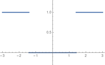
Behold, a continuous function.
And now things seem off. The graph doesn’t look continuous. But that’s because it jumps “at” \(\sqrt{2}\)—and in the rationals, that number doesn’t exist. So even though the function is continuous, it gives the outputs \(0\) and \(1\), but never anything in between; the Intermediate Value Theorem fails.
Even worse, the function has a derivative of zero everywhere. And looking at the graph, this makes sense, right? We can’t find any specific point where the function is increasing or decreasing; the tangent line at any point is horizontal. (Again, there should be a bad point at \(\sqrt{2},\) but since that number isn’t rational we don’t care.) And thus the value of the function changes, even though the rate of change is always zero. The Mean Value Theorem fails.
This function does satisfy the Extreme Value Theorem, but it’s not too hard to find other functions that don’t.
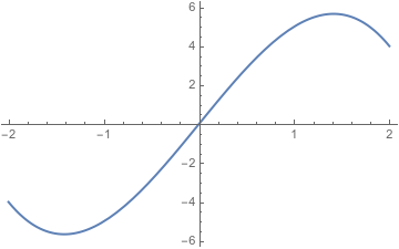
The graph of \(6x-x^3\) between \(-2\) and \(2.\) In the real numbers, it has a maximum at \(\sqrt{2};\) when restricted to the rational numbers, it has no minimum or maximum.
Now, this is all kind of dumb. The function \(f\) shouldn’t be continuous; there are obvious jumps in it! And the function \(6x-x^3\) has an obvious maximum in its graph. But that’s exactly the point. The rational numbers just aren’t good enough to do calculus, because obviously dumb and false things wind up being, technically, true. The function \(f\) is “continuous” because it jumps at an irrational number, and the function \(6x-x^3\) has “no maximum” because the maximum value happens at an irrational number. The rational numbers have gaps, and if we don’t fill in the gaps with real numbers, calculus just doesn’t work.
And while these examples talk about the rational numbers, we can also find examples that break in the algebraic numbers. They’re just way more annoying to describe, so I don’t want to write out the details.
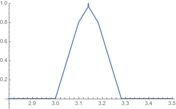
This is a continuous function that sends algebraic numbers to algebraic numbers but has no maximum in the algebraic numbers. I’m not going to try to define it here. I had to get help from three people to define it properly, and writing the code for the graph took half an hour. Please don’t ask me to explain it.
Whereof one cannot speak
There’s one more shot we have at avoiding all this nonsense. The rational numbers don’t work, and the algebraic numbers don’t work. But in this essay we described a new set of numbers, which contains all the algebraics and more, but is still countable: the computable numbers. Can we use these to do calculus, and avoid thinking about the uncountably many uncomputable reals?
Surprisingly, the answer is yes—sort of.
If we can give a recipe for \(x,\) and a recipe for \(y,\) then we can give a recipe for \(x+y\)—by saying \(“x+y”!\) We can do the same thing for subtraction, multiplication and division, so when we do algebra with computable numbers, the result is also computable. That means the computable numbers are a field.
The computable numbers are ordered, because they’re all real numbers, so we can compare two and see which one is bigger. They are not complete—if they were, they’d just be the real numbers. But they’re something almost as good: they’re “computably complete”.
Remember completeness means that any sequence that looks like it should converge does in fact converge; the real numbers are never just missing the number the sequence wants to converge to. But this isn’t true for the computable numbers. There are sequences of computable numbers that converge to uncomputable numbers.
However, I can’t give you any examples of those sequences. And in this case I’m not just being lazy; I really can’t give you an example. Because if I could describe a sequence of computable numbers that converges to \(x,\) then that sequence gives a recipe for computing \(x,\) and so \(x\) must actually be computable. And that means that every computable sequence of computable numbers converges to a computable number. Not every sequence will behave well, but every sequence we can actually describe will.
In the same way, none of the value theorems are technically true in the computable numbers. But they’re almost true. They’re computably true.
When we found rational functions that failed the value theorems, we did something extra: we described them using only rational numbers. (That’s why the condition was \(x^2>2\) and not \(x > \sqrt{2},\) for instance.) But for the computable numbers we can’t do that. There are functions from the computable numbers to the computable numbers where the value theorems fail, but those functions are themselves uncomputable. Any function that we can actually compute the results of will satisfy the value theorems. If we do anything even vaguely reasonable, everything will work the way we expect.
One must remain silent
So we could avoid the weirdness of the reals and stick to the computables. If we work in the reals, every number we actually talk about will be computable, so we don’t gain anything by allowing all the real numbers. And if we work in the computables, every function we want to think about will satisfy the value functions.
But there’s no reason to stay in the computables—it fundamentally doesn’t matter. We work in the reals because they give us precisely the tools we want.
Sure, we don’t want to deal with with arbitrary infinite decimals, and we certainly don’t deal with Dedekind cuts. But we don’t want to think about explicit computer programs for every number we ever use, either. What we want is the value theorems; what we want is a complete ordered field. And when we ask for that, without adding any restrictions, the real numbers are what pop out.
We shouldn’t think about the reals using their formal definition. We should think about what they do for us, the tools they allow us to use and the moves they allow us to make. The real numbers are a complete ordered field, and they give us the value theorems, so calculus works. And that’s all we want. We don’t need to make it more complicated than that.
But next time we’ll make it complex, instead.
Do you have comments, or questions? Are there other types of numbers you want to learn the story behind? Tweet me @ProfJayDaigle or leave a comment below.
-
We’re going to ignore the negative numbers here because they make everything more complicated in a boring and annoying way. I promise I could include them if I wanted to make this section even longer. ↵Return to Post
-
Fancy number theorists call this sort of thing a height. It’s a convenient way of putting as "size" on rational numbers so that there are only finitely many small ones, which is useful when we want to put things in order, or compute probabilities. ↵Return to Post
-
In part 1 we said rational coefficients, but this is the same thing. If you have an equation with rational coefficients, you can multiply through by the least common denominator and get an equivalent equation with integer coefficients. And assuming all the coefficients are integers is way more convenient for what we’re going to do here. ↵Return to Post
-
We could also pick 1, or 2, or 3, or 4, or 5, or 7, or 8, or 9; this isn’t a deterministic process. We just can’t pick 6. ↵Return to Post
-
There’s some slight weirdness here around the fact that \(0.99\dots~ = 1.\) But it’s not a real problem; don’t worry about it. ↵Return to Post
-
We could also stick it in the middle, or replace some element of the list we started with. But we can’t tack it on to the end, because this is an infinite list—it doesn’t have an end! ↵Return to Post
-
You might feel like this probability is obviously too big, and of course you’re right. But none of the argument depends on the specific number. I just want to keep the number small so it’s easier to think about what’s going on. ↵Return to Post
-
If this seems like a lot of symbols, you’re right! English has, like, thirty, and thirty is way smaller than infinity. But the lambda calculus, which is the mathematical formalism I linked, does in fact want an infinitely long list of symbols. Since this argument works either way, I’m letting the list be infinite. ↵Return to Post
-
If we give up on having an order, we can get "looping around" behavior, where repeatedly adding \(1\) gets us back to where we started. This shows up in modular arithmetic and finite fields, which I hope to discuss later in this series. But in an ordered field, this sort of looping isn’t possible, because adding \(1\) will always make a number larger. ↵Return to Post
Tags: math teaching calculus analysis philosophy of math