A Fictional History of Numbers, Part 4: Imagination, Complexity, and the Fundamental Theorem of Algebra

Welcome back to our survey of the different types of “numbers” that mathematicians work with, and what kind of questions lead us to study those numbers. This week we’re going to put a bow on the first collection of questions we asked and tie them all together.

In the first few essays in this series, we saw two different approaches to finding new types of numbers. But they gave us different—and overlapping, but distinct—sets of numbers. Today we’ll see what happens when we combine both techniques, and develop the complex numbers. This won’t finish our quest to find weird numbers that mathematicians care about; far from it. But it will finish one line of questions, and cover pretty much everything we normally see in high school algebra and calculus.

But before I start, I want to take a moment to thank everyone who has donated to my Ko-Fi account. Tips are never necessary, but always appreciated, and they really do make a difference and help me to keep writing essays like this one.

Building the complex numbers

The two approaches

In part 1, we started with the natural numbers, which are the basic numbers we use to count. Using basic arithmetic operations, we introduced negative numbers to get the integers, then fractions to get the rational numbers. We ended by asking all polynomial equations to have solutions, which gave us the algebraic numbers. These include square roots and cube roots of all the rational numbers, and also some stranger things like the solutions to \(x^5+x+3=0\). This gave us a set that was algebraically closed: any polynomial equation defined with algebraic numbers will have a solution that is an algebraic number. So algebraic tools couldn’t push us any farther.

In part 2 we asked a different question, about measurement and approximation. We wanted areas and lengths to all correspond to numbers, and this led to the idea of completeness, where any number we can approximate with rational numbers should actually exist. Completing the rational numbers gave us the real numbers. We might call this the analytic approach to extending the rationals, in contrast to the algebraic approach of part 1.

In part 3 we showed that not every real number is algebraic; in particular \(\pi\) is a transcendental number, which isn’t the solution to any polynomial equation. But more generally, we showed that the algebraic numbers are countable, which means we can describe any one of them with a finite amount of information, but the real numbers are uncountable, which means it takes an infinite amount of information to describe most of them. There aren’t just more real numbers than algebraic numbers; there are infinitely more.

But that doesn’t mean the real numbers cover everything! There are algebraic numbers that aren’t real numbers. And there are real polynomials that don’t have real solutions. So what happens if we start with the real numbers and do part 1 again? Can we get a field with the completeness of the reals, but also the nice algebraic closure of the algebraic numbers?

Keeping it unreal

How do we know there are algebraic numbers that aren’t real?

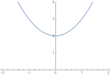
We can start with the quadratic polynomial equation \(x^2+1=0\). This is defined entirely with real numbers. But when we graph the function \(x^2+1\), we see it doesn’t cross the \(x\)-axis, which means that \(x^2+1=0\) doesn’t have a real solution.

We maybe should have expected this. We know that \(\sqrt{2}\) is real, because we can find a rational numbers whose squares are between \(1\) and \(2\), or \(1.9\) and \(2\), or between \(1.99999\) and \(2.\) That gives us a sequences of numbers that approximates \(\sqrt{2}\), and thus \(\sqrt{2}\) must be real. But we can’t do the same trick for \(−1\): no rational number has a square less than zero, so we can’t find anything that’s close to the square root of \(-1\).

But we can see this more directly by using the core principles of the real numbers: they’re a complete ordered field. Since they’re ordered, that every (non-zero) number must be either positive or negative. Since they’re an ordered field, the product of two positive numbers must be positive, and the product of two negative numbers must also be positive.

So suppose we have a number \(i\) that solves this equation. Then \(i^2 = -1\), which means \(i\) can’t be positive, and also can’t be negative. It’s clearly not zero. So it can’t be a real number at all. But it’s definitely algebraic: it’s the solution to \(x^2+1=0\).

Can we find other non-real algebraic numbers? Sure! There’s \(2i\) and \(3i\) and \(1+i\) and…. We can use \(i\) to build lots more non-real numbers.

But that’s it. It turns out that if we take the real numbers, and then add in everything we can build with the number \(i\), we have all the algebraic numbers. And in fact we have the solution to any polynomial we can write down with real numbers. This gives us everything we could ever want.¹ But to see why this gets us everything, we’ll need to take a bit of a detour

Imaginary and complex numbers

We want to look at all the numbers we can build by combining the real numbers and \(i.\) These numbers will all look like \(a + bi\) where \(a\) and \(b\) are real numbers.² And we call the set of all these things the complex numbers, abbreviated \(\mathbb{C}.\) If we have a complex number \(z = a + bi\) then we say the real number \(a\) is the real part and the real number \(b\) is the imaginary part.

Remember our goal was to extend the real numbers to something algebraically nice. So we should start my making sure that we can still do arithmetic operations—that complex numbers are a field. Now, addition and subtraction are fine, since can use the rules \[ \begin{aligned} (a+bi) + (c+di) & = (a+c) + (b+d) i \\ (a+bi) - (c+di) & = (a-c) + (b-d) i . \end{aligned} \] Multiplication is also pretty straightforward. By FOILing we get \[ \begin{aligned} (a+bi)(c+di) & = ac + adi + bci + bdi^2 \\ & = ac + adi + bci + bd(-1) \\ & = (ac - bd) + (ad +bc)i \end{aligned} \] so if we multiply two complex numbers, we get another.

Division is a little trickier; we don’t have a good way to distribute something like \( \frac{a+bi}{c+di}. \) Here we need to be clever, and maybe start by asking a new question that introduces a second big idea.

We defined \(i\) to be the square root of \(-1\). That is, \(i^2=-1\) is the definition of the number \(i.\) But what happens if we square the number \(-i\)? We have \[ (-i)^2 = (-1)^2 (i)^2 = 1 \cdot (-1) = -1. \] So we have two different numbers that both satisfy our equation \(x^2 = -1.\) How do we know which is the “positive” \(i\), and which is the “negative” \(-i\)?

And the answer is that there’s no real difference! A positive number like \(4\) has two square roots, \(2\) and \(-2\), and since they’re both real numbers one is positive and the other is negative. A negative number like \(-1\) will also have two square roots, but since they aren’t real numbers, neither one of them is actually positive. We just pick one to call \(i\), and call the other one \(-i\)—but it doesn’t matter which one is which. And that means that if we swap \(i\) and \(-i\), nothing else should change. Thus we can define an operation called complex conjugation by the rule \[ \overline{a + bi} = a - bi. \] This operation swaps \(i\) with \(-i,\) without changing anything else about our number.³

But the complex conjugate has another useful property. What happens if we multiply a number by its own conjugate? We get \[ \begin{aligned} (a+bi) \overline{(a+bi)} &= (a+bi)(a-bi) \\ &= a^2 +abi - abi - b^2 i^2 \\ &= a^2 - b^2 (-1) \\ &= a^2+b^2. \end{aligned} \] If we multiply any complex number by its conjugate, we get a real number—and in fact, a positive real number, as long as we didn’t start with 0.

And this gives us a way to complex-number divisions, by turning them into real-number division: \[ \begin{aligned} \frac{a+bi}{c+di} & = \frac{a+bi}{c+di} \frac{c-di}{c-di} \\ & = \frac{ (ac +bd) + (bc - ad)i}{c^2 + d^2} \\ & = \frac{ac+bd}{c^2+d^2} + \frac{bc-ad}{c^2+d^2} i. \end{aligned} \] So we can in fact divide by any non-zero complex number. This means we can do basic arithmetic, and thus the complex numbers are a field.

And like the real numbers, they’re complete. The simplest way to think about this: we can think of a complex number \(z = a +bi\) as a pair of real numbers \(a\) and \(b\). So a sequence of complex numbers is basically just two sequences of real numbers, and we know that sequences of real numbers behave well. So any complex number that we can approximate has to actually exist; there aren’t any holes.

So while the reals are the unique complete ordered field, the complex numbers are a complete unordered field, which contains all the reals. And by giving up the order, we hope to get something else: every complex polynomial has a complex number solution. Once we take the real numbers and add in \(i\) there’s nothing left to algebraically add.

But it’s not obvious why that’s true. How do we know there’s not some polynomial equation we haven’t thought of, that doesn’t have a solution even in the complex numbers? To answer this, we need to turn to geometry.

Complex Geometry

The complex plane

If we have a pair of real numbers, we can graph it on a plane, using the first number for the horizontal coordinate and the second number for the vertical coordinate. But a complex number \(z = a +bi\) is a pair of real numbers. And that means that, just like we can think of the real numbers as forming a line:

we can think of the complex numbers as forming a plane:

There are a lot of geometric ideas we can poke at here; for instance, complex numbers give us a useful way to talk about angles that I’m not going to talk about here, since it doesn’t help answer our current question.

But distances and sizes will be extremely useful. So let’s think about those: if we have a number \(z = a+bi\), let’s figure out how far away from the origin at \(0\) it is. The \(x\)- and \(y\)-coordinates are \(a\) and \(b\), so we have a triangle with side lengths \(a\) and \(b\). By the Pythagorean theorem, the length of the hypotenuse, and thus the distance from the origin, is \(\sqrt{a^2+b^2}\).

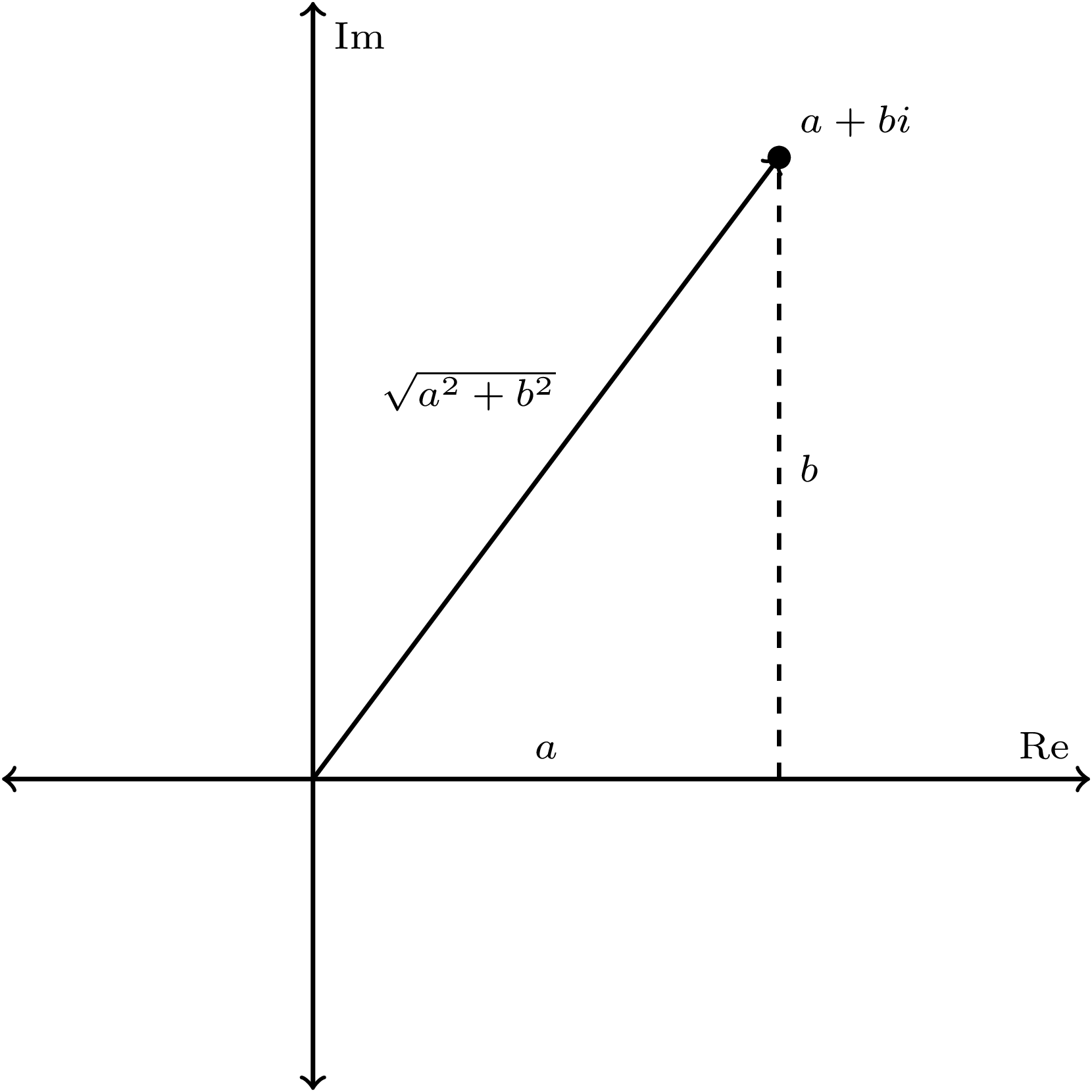
So far, we haven’t used the fact that we have complex numbers running around. But if we remember the calculations we did with the complex conjugate, we might notice that \[ a^2+b^2 = (a+bi)(a-bi) = (a+bi)\overline{(a+bi)}. \] So we can rewrite our distance formula: if we have a complex number \(z\), the distance from the origin is \(\sqrt{z \cdot \overline{z}} \). We call this the modulus or absolute value of the number \(z\), and write it \(|z|\). It’s one of the most important operations we can do with complex numbers.

Specifically, it allows us to talk about sizes. Because the complex numbers aren’t ordered, we can’t directly compare numbers like \(3-4i\) and \(1 + 3i\); neither one is greater than the other. But once we graph them it’s visually clear that \(3-4i\) is much further from \(0\) than \(1+3i\) is, and in that sense it’s definitely “bigger”.

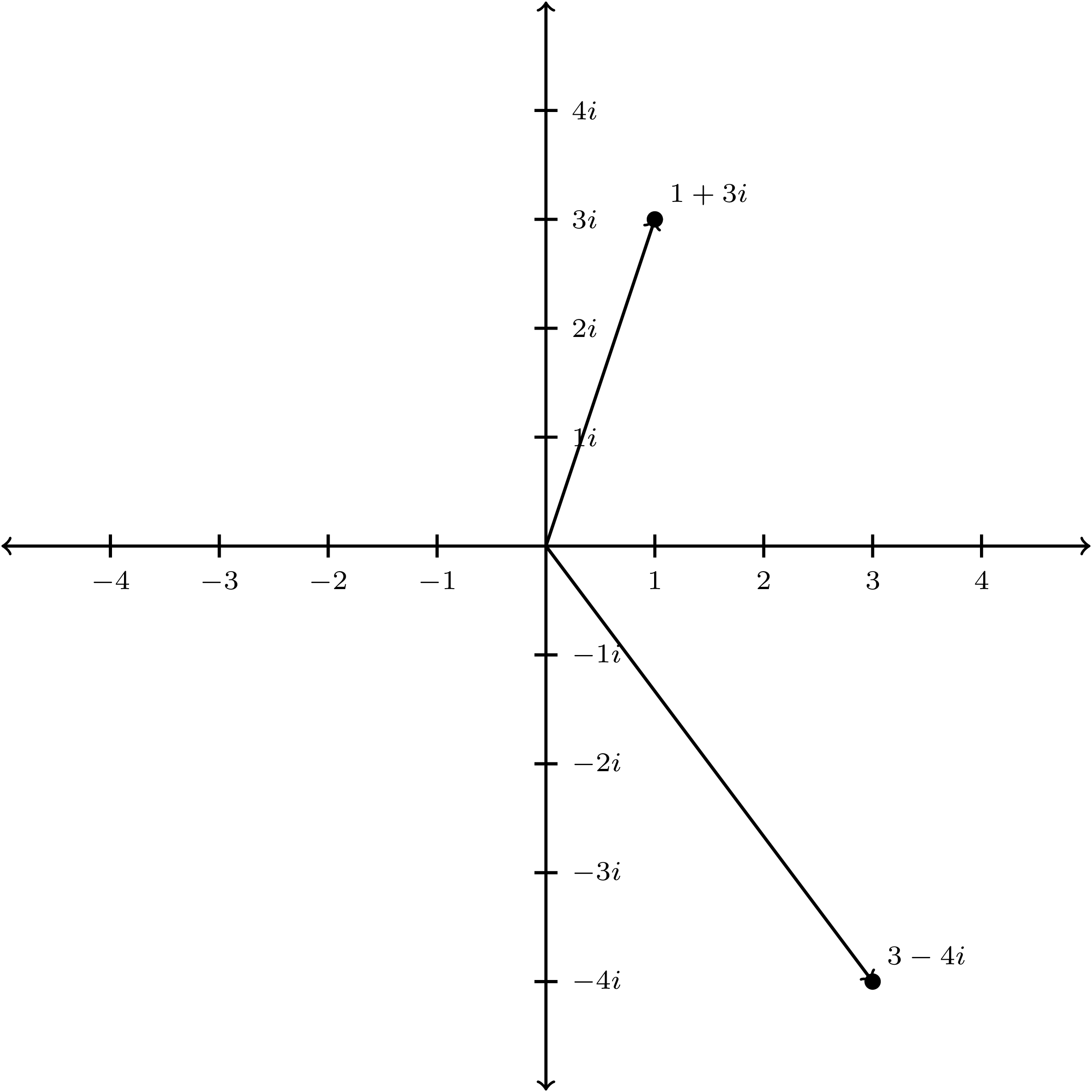
The modulus lets us compute this numerically: \[ \begin{aligned} | 3 - 4i | & = \sqrt{3^2 + 4^2} = \sqrt{25} = 5 \\ | 1+3i | & = \sqrt{1^2 + 3^2} = \sqrt{10} \approx 3.16 \\ \end{aligned} \] and so the first number is in this sense “bigger” than the second.

This size computation allows us to do a few things. First, we need it to do geometry, since it allows us to compute distances: the distance between \(z\) and \(w\) \( |z-w|\), the modulus of the difference. And then that lets us talk about “completeness” more precisely. Completeness tells us that when all the points in a sequence get close together, they must have some limit; for that to make sense, we need to know what “close” means!

And importantly for us, the modulus lets us talk about maximum values for functions. In the real numbers this is simple to talk about: we’re looking for the greatest possible output. But a function that outputs complex numbers can’t really have a maximum, because the outputs aren’t ordered! But instead we can look for the “biggest” output, where the modulus is greatest. Since the modulus is always a (positive) real number, this is a question that makes sense.

And once we investigate the maxima of complex functions, we get one of the most surprising results in all of complex analysis.

The Maximum Modulus Principle

In the real numbers we had three key theorems in our “value pack”. One was the Extreme Value Theorem, which says that a continuous function on a closed interval has a maximum and minimum value. This doesn’t quite work in the complex numbers, because the lack of order means we lack both maximum outputs, and also “intervals”.

A real interval is one-dimensional and doesn’t make sense in the complex plane.

But it’s basically true, after we tweak it. Instead of a closed interval, we want to have a closed and bounded region, which you can think of as a loop and everything inside of it, very much including all the points on the loop. And we need to look for the greatest modulus, instead of the “greatest complex number”. But after we make those tweaks, we can restate the Extreme Value Theorem: a continuous function on a closed and bounded region has a maximum (and minimum) modulus.

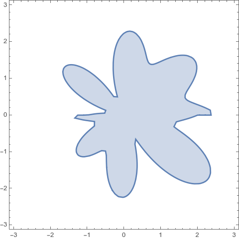A closed region in the complex plane. The outer blue boundary is included.

In fact, we can get even more than that. A real function on the plane has to have a maximum, but that can happen basically anywhere, without restrictions.

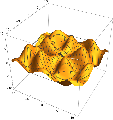
Some real-valued functions have lots of local maxima all over the place.

But a complex function, if it has a derivative, is much more restricted. The maximum modulus principle says that \(|f|\) doesn’t just have a maximum somewhere in the region; the maximum has to occur on the boundary of the loop. In fact, unless the function isn’t totally constant, the maximum value can only occur on the boundary. If we have a point on the inside of the loop, we can always get a bigger modulus by moving in some way towards the boundary, so there aren’t even local maxima on the inside of the region.

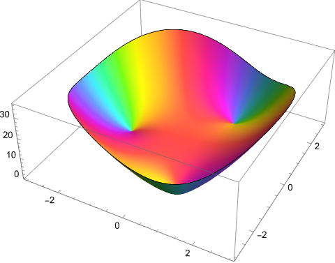The height in this graph gives the modulus of the output, and color tells us the angle. If you ignore color this graph looks extremely boring—which is the point.

This has widespread and surprising implications. One of the most famous is that if a complex function is differentiable and bounded—meaning there is some maximum modulus the function can output, no matter the input—then it has to be constant.

And that’s really restrictive! A differentiable real function can easily be bounded without being constant:

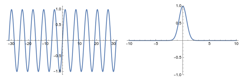The functions \(\sin(x)\) and \(e^{-x^2}\) are differentiable, bounded, non-constant real functions.

but a differentiable complex function cannot. Either it has only one possible output, or the outputs go to infinity. And this sort of behavior leads to what some mathematicians have jokingly called the only theorem of complex analysis:

Let \(f\) be a complex differentiable function with any interesting properties whatsoever. Then \(f\) is constant.

In truth, there’s a lot more to the calculus of complex numbers than that; and I could hang out all day talking about cool weird tricks. Like, we can use complex numbers to compute the integrals of purely real-valued functions that are too tricky to solve over just the real numbers, and that’s really cool and also kind of obnoxious.

But that’s not what we’re here for. We just wanted to take the real numbers, and add in everything we needed to make all our polynomial equations have solutions. And now we’re ready to prove that \(i\) is the only thing we had to add.

The fundamental theorem of algebra

Theorem: Any non-constant polynomial equation with complex coefficients has a complex number solution.

Proof: Suppose we have some complex polynomial \(f(z)\) that doesn’t have any roots. We start by drawing big loop in the complex plane—big enough that \(|f(z)| > |f(0)|\) for every \(z\) on the boundary of the loop. We know we can do this because a polynomial will always get very big when the input gets very big.⁴

Then the maximum value of \(|f(z)|\) happens on the boundary of the loop, but the minimum has to happen on the inside of the loop, since \(0\) is on the inside, and \(|f(0)|\) is smaller than any value we get on the boundary. (It’s not necessarily the minimum itself; there could be points that give even smaller values. But we know the minimum can’t be on the boundary because all the boundary points give big values.)

So we know that \(f\) is a differentiable function, with a maximum on the boundary of the loop, and a minimum on the inside. We can also define the function \( \frac{1}{f} \), which will flip this. When \(|f|\) is big, then \(\frac{1}{|f|}\) will be small, and vice versa; so \(\frac{1}{|f|}\) has its minimum on the boundary of the loop, and its maximum on the inside.

But we also know something else. Since \(f\) has a derivative, we know that \( \frac{1}{f} \) also has a derivative, so the maximum modulus principle applies: the maximum value of \( \frac{1}{|f(z)|} \) must occur on the boundary of the loop. But we just said that the maximum has to occur on the inside of the loop; something has gone wrong.

The culprit is our assumption that we could actually compute the function \(\frac{1}{f}\) everywhere inside the loop. That’s only true if \(f(z)\) is never zero, since we can’t divide by zero. Because that assumption led to a contradiction, we know \(f(z) = 0\) for some value of \(z\)—so there is a solution to the equation we started with. ∎

The end of one road

And this means that the complex numbers are sort of the end of this series of questions. In part 1 we started with the natural numbers, wanted to do algebra to them without worrying, and wound up with the algebraic numbers. In part 2 we started with the natural or rational numbers, wanted to do geometry and make approximations, and found the real numbers.

The algebraic numbers weren’t complete, meaning they’re inadequate for doing geometry and calculus. The real numbers are perfect for doing calculus, and are great for approximations, but they’re not algebraically closed—there are those pesky polynomial equations like \(x^2+1=0\) that don’t have solutions.

Now we can combine the two ideas, and get the complex numbers. They’re complete, so we can do geometry and calculus. They’re algebraically closed, so we can do whatever algebra we want. And they’re in many ways the best tool for doing both algebra and geometry.

But we did lose something when we moved to the complex numbers: we lost the ordering, and with it we lost some of our key calculus theorems from the reals.

• The Intermediate Value Theorem says that if a continuous real function can output two distinct numbers, it can also output anything in between them. In the complex numbers this isn’t true, because we have two dimensions and so we can go around. In the real numbers, to get from \(-1\) to \(1\) we have to go through \(0\); in the complex numbers we can go through \(i\) instead.

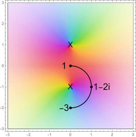The function outputs zero at the Xs. This path takes the output from \(1\) to \(-3\) without ever passing through zero.

• The Mean Value Theorem says that if we have a differentiable real function on a closed interval, the average speed is equal to the derivative at some point. This fails in the complex numbers for the same reason the intermediate value theorem does; we can get from a speed of \(30\) mph to a speed of \(60\) mph without ever going \(45\) mph, because we can travel at \(45+i\) mph instead. (Physically this may or may not be meaningful, but mathematically it works.)

  But this time we can recover an important chunk of the result. The Mean Value Theorem tells us speed limits work: if our speed is never higher than sixty miles per hour, we can’t possibly travel more than sixty miles in one hour. And we can still get that principle in the complex numbers, because the modulus of the distance we travel has to be less than the modulus of the time we spend, times the modulus of the speed. So we can save the tool we really care about—but only by shifting things back to the real numbers.

• We already talked about the Extreme Value Theorem. In this case the complex numbers have an even stronger version than the reals did, in the Maximum Modulus Principle; it’s just so strong that it makes things really weird.

So of our three key calculus theorems, one is basically true but very strange, one is salvageable in a much weaker form, and one is just gone. And that makes the complex numbers awkward for doing calculus, in the sense we normally mean calculus. They’re not good for talking about speeds, or rates of change, or anything like that—at least not directly.

On the other hand, they’re great for doing algebra and geometry (and algebraic geometry). And there are all sorts of problems that don’t start out in the complex numbers, but can be transformed into complex-number questions, where we can throw our extremely powerful tools at them. (And then hopefully translate those answers back into real-world information!)

But we’re not going to talk about that here. My promise in this series was I would pose reasonable questions, and show you how answering them gives us new numbers; and that’s what we’ve done. We wanted to expand the natural numbers using basic operations, and now we can’t expand any further. We wanted a field that is complete and algebraically closed, and we got it. Until we find a new question, we can rest content.

I’m done with this line of questions; but I’m not at all done with this project! I hope to talk about quaternions and octonions, finite fields and modular arithmetic, \(p\)-adic numbers, transfinite numbers, infinitesimals, and function fields. Let me know what you’d like to hear about—tweet me @ProfJayDaigle or leave a comment below.