Hypothesis Testing and its Discontents, Part 1: How is it Supposed to Work?
In my last post on the replication crisis, I mentioned the basic ideas of statistical hypothesis testing. There wasn’t room to give a full explanation in that post, but hypothesis testing is worth understanding, since it’s the foundation of most modern scientific research. It’s a powerful tool, but also incredibly easy to misunderstand and misuse.
This post is the first part of a three-part series explaining what hypothesis testing is and how it works. In this essay I’ll talk about the way hypothesis testing developed historically, in two rival schools of thought. I’ll explain how these two methodologies were originally supposed to work, and why you might (or might not) want to use them. In Part 2 I’ll talk about how we do significance testing in practice today, and how that often goes wrong. And in Part 3 I’ll talk about alternatives to hypothesis testing that can help us avoid replication crisis-type problems.
Choose your question
Perhaps the most important step in using math to solve real-world problems is figuring out precisely what question you want to ask. Now, there’s a sense in which this process isn’t mathematical. Math can’t tell you, say, whether you want your clothing to be more comfortable or more stylish. No amount of math can tell you how you value inequality versus growth, or whether you’re willing to risk major side effects from an experimental medical treatment.
But math can help you figure out what question you’re asking, by clarifying exactly what questions you could be trying to answer, what their implications are, and what options you have for answering them. The history of hypothesis testing is a debate between people trying to answer different questions, but also a debate about which questions are the most fruitful to ask. Do we want to test a scientific principle? Record a precise measurement? Make a decision?
The statistical tools we use today were developed by specific people,1 at specific times, to answer specific questions. So I want to start off by asking some of those specific questions, and see how early statisticians would approach them and what ideas they developed in response.2 After we’ve seen how Fisher’s significance testing and the Neyman-Pearson hypothesis testing framework worked in their original contexts, we can talk about what questions each tool is best suited to answer, and what types of question neither tool can really handle.
Fisher’s Significance Testing
Are You Surprised?
In 2016 I got a new car with a fancy new electronic system. And one of the new features was a meter that kept track of my gas mileage. It was fun to watch the mileage adjust as I was driving. (And I may have gotten a little obsessed with trying to eke out another tenth of a mile per gallon by driving funny.)
But how accurate is that mileage number? In 2019 my friend Casey suggested an experiment to me and I decided to try it. For several months, every time I filled up my gas tank, I recorded the mpg number from my car dashboard. I also recorded the number of miles I’d driven and the number of gallons of gas I’d used, which let me calculate the mpg directly.
| Miles Driven | Gallons | Calculated MPG | Dashboard MPG | Difference |
|---|---|---|---|---|
| 340.7 | 10.276 | 33.2 | 34.2 | 1.0 |
| 300.1 | 8.97 | 33.5 | 34.7 | 1.2 |
| 232.6 | 8.04 | 28.9 | 29.0 | 0.1 |
| 261.8 | 8.5 | 30.8 | 31.1 | 0.3 |
| 301.3 | 9.316 | 32.3 | 32.5 | 0.2 |
| 505.1 | 15.127 | 33.4 | 34.8 | 1.4 |
| 290.3 | 9.814 | 29.6 | 30.3 | 0.7 |
| 290.2 | 8.566 | 33.9 | 34.9 | 1.0 |
| 294.9 | 9.005 | 32.7 | 32.8 | 0.1 |
| 301.4 | 9.592 | 31.4 | 32.0 | 0.6 |
| 230.9 | 7.643 | 30.2 | 32.0 | 1.8 |
| 269.2 | 8.644 | 31.1 | 30.8 | -0.3 |
| 267 | 8.327 | 32.1 | 32.6 | 0.5 |
| 319.7 | 9.42 | 33.9 | 34.7 | 0.8 |
| 314.3 | 9.868 | 31.9 | 33.3 | 1.4 |
| 264.4 | 8.693 | 30.4 | 31.7 | 1.3 |
| 273 | 9.229 | 29.6 | 30.4 | 0.8 |
| 320.2 | 9.618 | 33.3 | 33.3 | 0.0 |
These numbers show that my car reported a better mileage than I actually got almost every time. Out of eighteen measurements, my car overestimated sixteen times, underestimated once, and was accurate to one decimal place once. But was this tendency toward overestimation a coincidence? Is my car’s mileage calculation biased high, or did I just get weirdly unlucky?
We can try to get a sense of how easily this could have happened by chance. We took eighteen measurements, and sixteen of them were high. (One was a tie, but we’ll be generous and count it as “not high”.) If the car is equally likely to guess high or low, this is like flipping a coin eighteen times and getting sixteen heads. That’s pretty unlikely: the probability is about \(0.0006\), or \(0.06\)%, or about one in \(1700\). It’s still possible that my car is unbiased and I just got unlucky. But if so, I was extremely unlucky.
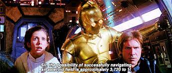
But still only half as unlucky as Han Solo’s enemies.
What is a significance test?
We call this approach a significance test. This approach was developed by Ronald Fisher, following up work by Karl Pearson and William Sealy Gosset.
We start by formulating a null hypothesis that represents some form of “expected” behavior, which we call \(H_0\). In this case, I expected3 my car to correctly measure my gas mileage, without consistent bias in either direction. There are a few ways to make that expectation mathematically precise; in the example above, my precise hypothesis was “an overestimate is just as likely as an underestimate”, or more formally, \(P(\text{overestimate}| H_0 ) = 0.5 \).
(There are other ways to formalize my expectations here. I ignored the size of the errors, and just looked at whether the measured mileage was better or worse than the mileage I calculated. But with a more complicated statistical tool called a paired \(t\)-test we can use the exact numbers to get a bit more information out of our measurements. When I do this, I get a \(p\)-value of \(0.00004\), or \(0.004\)%—an order of magnitude lower than my first figure.)
Once we have a null hypothesis, we compute how unlikely the measurement we actually got would be, if we assume the null hypothesis is true. And if that sentence looks confusing and grammatically tangled, there’s a reason for that: while this process is absolutely unambiguous mathematically, it has nested “if-then” statements that are hard to think clearly about and don’t translate easily into English. In mathematical notation, we want \( P( \text{measurement} \mid H_0 ) \), which we can read as the probability of seeing our measurement given the null hypothesis.
There are a couple of subtle points here, so I want to be super explicit and run them into the ground. The first is that we need to be careful about what we mean by “how unlikely our result is”, because any specific result is extremely unlikely. The odds of getting the exact sequence I got in my experiment—HHHHHH HHHHHT HHHHHT—are exactly \(1\) in \(2^{18}\), because that specific sequence isn’t special. If you pick any specific sequence, whether it’s all heads like HHHHHH HHHHHH HHHHHH, or half-and-half like HTHTHT HTHTHT HTHTHT, or something totally random like HHHTHT HHHHTT HTTHTT, the odds of getting those exact flips in that exact order is \(1\) in \(2^{18}\).
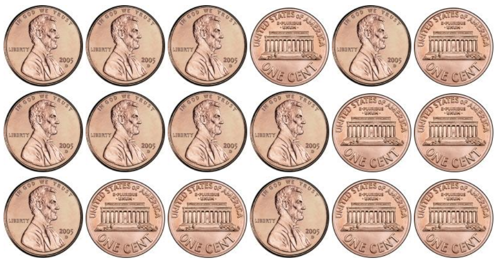
The probability of getting these exact flips in this exact order is \(1\) in \(2^{18}\), or about \(0.000004\).
But that doesn’t tell us anything useful! Fortunately, in the context of hypothesis testing, we can do something smarter. It doesn’t really matter what order we get the heads in; it just matters how many we get, because that tells us how often the car is overestimating my mileage. So we can compute the odds of getting sixteen heads in any order. And getting seventeen heads would be even more unlikely, so we include that as well; so what we wind up computing is the odds of getting \(16\), \(17\), or \(18\) heads. That’s how I got the number \(0.0006\) earlier.
We say that we want to compute the chance of getting a result at least as bad as what we got. But that requires us to decide what counts as “better” or “worse”; and that depends on what question we’re actually trying to ask. In this context, I’m testing the null hypothesis that my car underestimates as often as it overestimates, so I can basically order the possible results from “most overestimation” to “most underestimation” and find the probability of overestimating at least as often as my car actually did.
What we don’t learn
Another subtle point, but an absolutely vital one, is that the \(p\)-value does not tell us how likely the null hypothesis is to be true. When we say that \(p = 0.0006\) that does not mean that there’s only a \(0.06\)% chance that my car is accurate! It just measures how unusual my evidence is, if the null hypothesis is true.
Often the question we really care about is how likely the null hypothesis is to be true. There are in fact ways to try to address that directly, which I’ll discuss in Part 3 of this series. But answering that question requires a lot more information than we usually have; Fisher’s significance test doesn’t try. It just assumes the null hypothesis is true, and tells us how weird that makes the result look.
Significance testing does numerically measure the strength of the experimental evidence we got: the lower the \(p\)-value, the stronger our evidence. But it doesn’t try to account for any other evidence we have, whether against the null hypothesis or for it. If I get a coin from the bank, flip it ten times and get ten heads, I get \(p \approx 0.001\) for the null hypothesis that it’s a normal coin. But I still expect it to be normal, because most coins are. And if I pick it up and see that it has a normal “tails” side, I’ll be really confident that I just got weirdly lucky4.
And that’s why the analysis of my gas mileage above didn’t really have a firm a conclusion. We got a \(p\)-value of \(0.0006\), and determined: “huh, that’s kinda funny”. Either our null hypothesis was false, or something extremely unusual happened. But the math doesn’t tell us which of those two things to believe.
And in the case of my car, it doesn’t need to. On the one hand, I’m not all that surprised if the mileage calculator is a little wrong; the super-low \(p\)-value just reinforces what I already suspected. And on the other hand, I’m not really going to do anything different if my mileage is half an mpg lower than my dashboard says. I’m not going to sue Honda, or lead an activist campaign, or try to raise awareness about faulty mileage estimates.
But if I really cared, I could run more experiments. I got \(p = 0.0006\) in my first experiment; but I could do the experiment again. If I get \( p = 0.31\) next time, maybe I should assume the first result was just a fluke. But if I get \(p = 0.0003\) and then \( p = 0.0008\) I’ll see a pattern. And that pattern would make a convincing argument that my car is lying to me.

In “The Arrangement of Field Experiments”, Fisher writes that “A scientific fact should be regarded as experimentally established only if a properly designed experiment rarely fails to give this level of significance”. (Italics in the original.) That is, no one experiment should convince us of anything. Instead, we should believe our results when we can reliably design experiments that give the same results (which is arguably the point that we pass from science to engineering).5
But that’s a slow, grinding, painstaking process. And it still doesn’t give us a rule for when to pull the trigger! We just gradually believe the null hypothesis less and less as we collect more data. That’s perfectly fine for doing basic science—maybe even ideal.
But what if the stakes are higher, and more immediate? Sometimes we need to make a real decision, now, with the data we have. So what do we do?
Neyman-Pearson Hypothesis Testing
Time to make a choice
Suppose we’re studying a new drug, which we hope will prevent deaths from cancer. We can collect data on how effective the drug seems to be in trials, but just reporting a \(p\)-value isn’t enough. At some point we have to make a decision: should we give people the drug, or not? And Fisher’s methods don’t answer that.6
Jezry Neyman and Egon Pearson (the son of Karl Pearson) decided to attack that question head-on. They began by observing that there are two different mistakes we could make, which they called “Type I” and “Type II” errors.
These names are infamously unmemorable, but in their original context they make perfect sense: whichever mistake we most want to avoid is the “first type” of mistake. For drug testing, there’s a widespread consensus that it’s worse to prescribe a drug that doesn’t work, or has nasty side effects, than it is to withhold a drug that works as expected.7 So the Type I error would be prescribing a drug that doesn’t work, and the Type II error would be failing to prescribe a drug that does work. This means we can take “the drug doesn’t work” as our null hypothesis \(H_0\). But we can contrast our null hypothesis with a specific alternative: that the drug does, in fact, work. We call this our “alternative hypothesis” \(H_A\). And we get the following classic chart:
| Null Hypothesis is false (Drug works) |
Null Hypothesis is true (Drug doesn’t work) |
|
|---|---|---|
| Give the drug (Reject the Null) |
Correct decision “True Positive” |
First, worse error (Type I Error) “False Positive” |
| Don’t give the drug (Don’t Reject) |
Second, less bad error (Type II Error) “False Negative” |
Correct Decision “True Negative” |
This leaves us with a problem. There are two different mistakes we could make. And without getting better data, we can only reduce the Type II errors by increasing the Type I errors: if we’re more generally willing to say “yes, prescribe the drug”, we’ll say “yes” more often when the drug works, but also when it doesn’t. We need to strike some sort of balance between the two risks. But how?
There’s no abstract, mathematical answer to this question; it depends on the specific, practical consequences of the decision we’re making, and how much we care about the specific trade-offs in play. We already said that a Type I error is worse than a Type II error—but by how much? Is it two times as bad? Five? Ten? We have to decide exactly how we weigh the two risks against each other.
In drug testing, a Type I error means spending money on drugs that don’t work and might hurt people. A Type II error means people don’t get treatment that would help them. If a disease is really bad, we’re more willing to make Type I errors, because a drug that might kill you compares favorably to a disease that definitely will. If a drug is really expensive, or has bad side effects, we might be more willing to make Type II errors, because people will be hurt more by letting a bad drug slip through. And there are dozens more factors like that that we have to weigh against each other.
Once we’ve decided how we want to balance these risks, we can define a threshold for our experiment. If our data falls crosses that threshold we prescribe the drug; if the data doesn’t cross the threshold, then we don’t. And that’s our decision.
The risk of error
All this setup leaves us with a pair of numbers that describe the trade-offs we’ve made. The rate of Type I errors is \(\alpha\), which tells us: if the drug doesn’t work, how likely are we to prescribe it? Its mirror is \(\beta\), the rate of Type II errors. This tells us: if the drug does work, how likely are we to withhold it? 8
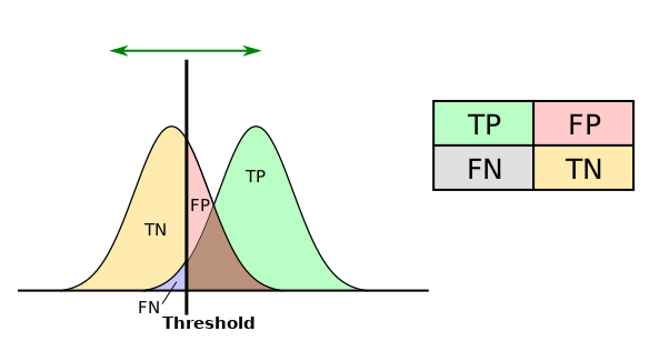
We give the drug if our measurement is bigger than the threshold. If the drug works, we’ll get a result from the right (green) bell curve; if it doesn’t, we’ll get a result from the left (yellow) one.
ROC_curves.svg: Sharprderivative work: נדב ס, CC BY-SA 4.0, via Wikimedia Commons
(You’ll often see \(\alpha\) referred to as the “false positive rate” and \(\beta\) as the “false negative” rate, but that’s a little inexact. In modern practice, the null hypothesis is almost always “there is no effect”, but this isn’t necessary to the framework. If we want to err on the side of prescribing the drug, then “the drug works” would be the null hypothesis and “no it doesn’t” would be the alternative. In that case, rejecting the null would be a negative result and a Type I error would be a false negative.)
But through all this, we have to be careful about what question we’re asking, and whether our methods can answer it. Naively we might want to ask something like “how likely is it that this drug works”, but Fisher, Neyman, and Pearson all would have agreed that that’s an incoherent question that can’t really be answered.9 (And even if you believe it’s a coherent question, it’s still not an easy one.)

Instead, the probabilities we computed are both conditional: if the drug doesn’t work, how likely are we prescribe it? And if the drug does work, how likely are we to withhold it? We can use those probabilities to make the best possible decision, given the information we used and the assumptions we made. But we can’t compute the probability that our decision is correct, because that’s just not the question that the Neyman-Pearson method can answer.
Don’t tell me what to think!
In fact, the Neyman-Pearson method is even less able to answer that than the Fisher method. Fisher can’t tell us the probability that we’re right, but it’s at least an attempt to figure out whether we’re right, by measuring our experimental evidence against the null hypothesis. But Neyman-Pearson doesn’t even try to tell us whether the drug “really works” or not. It just tells us what we should do.
And it is very possible to believe that a drug probably works and is safe, but also that we’re not sure enough to go around prescribing it; it’s equally possible to believe a drug probably doesn’t work, but it’s cheap and harmless so we might as well give it a shot. Neyman himself wrote, in his First Course in Probability and Statistics:
[T]o accept a hypothesis \(H\) means only to decide to take action \(A\) rather than action \(B\). This does not mean that we necessarily believe that the hypothesis \(H\) is true. Also, [to reject] \(H\) means only that the rule prescribes action \(B\) and does not imply that we believe \(H\) is false.
Researchers talk about the difference between statistical significance and practical or clinical significance, but in the true Neyman-Pearson setup, practical and statistical significance should be the same. Sure, if your measurements are precise enough, you can detect an effect that’s too small to matter. Conversely, a small pilot experiment can provide exciting, suggestive data without conclusively establishing any facts. But Neyman-Pearson is designed to choose a significance threshold \(\alpha\) to optimize decision-making, and that means that the statistical threshold must be a practically significant threshold.
If we’re trying to make an optimal decision based on limited information, Neyman-Pearson is about the best we can do. And that’s a pretty plausible description of a lot of medical studies. Phase III drug trials are slow, difficult, and expensive; we’re not going to run the whole thing over again just to check. We need a threshold for deciding whether to approve a drug or not, with the information we have; and that threshold is necessarily a practical one.
But scientific research isn’t generally about single isolated decisions; it’s a search for knowledge, an attempt to figure out what’s true and what isn’t. Neyman-Pearson very specifically wasn’t designed to answer questions about truth, but we try to use it to do science anyway. I’ll talk about how exactly that works (and doesn’t work) in Part 2 of this series; but (spoilers!) it works out awkwardly, and the mismatch between what Neyman-Pearson does and what we want it to do is a major contributor to the replication crisis.
Making promises
The Neyman-Pearson method doesn’t tell you what to believe, but it does make a very specific promise: if you set your significance threshold to \(\alpha =5\)%, then your false positive rate will be \(5\)%. This is a statistics theorem, so it really is guaranteed—if you set everything up correctly.

But that guarantee only applies to the threshold you set before you saw the data. If you run your experiment, do your analysis, and compute \(p = 0.048\), then your result is significant, and the background false positive rate is \(5\)%. But if you run your experiment, do your analysis, and compute \(p = 0.001\), then your result is significant, and the background false positive rate is still \(5\)%. The false positive rate doesn’t get lower just because the \(p\)-value does.
Huh? Isn’t \(p = 0.001\) much stronger evidence than \(p = 0.048\)?
In one sense, yes. That’s what Fisher tells us. But Fisher doesn’t make decisions, and doesn’t make this statistical guarantee. It’s a different tool that answers a different question.
Neyman-Pearson does make a guarantee, but that guarantee is very specific. If you run a hundred experiments where the null hypothesis is true, you’ll only reject about five times. (And you get the lowest possible \(\beta\), the fewest possible false negatives, compatible with that false positive rate.) But that’s all you’re guaranteed.
And in particular, if the null hypothesis is true then all \(p\)-values are equally likely. So if you do a hundred experiments, you should expect one of them to give you \(p=0.95\), and one to give \(p = 0.05\), and one to give \(p=0.01\). And that \(0.01\) isn’t, mathematically, special. It’s just one of the five false positives you expect.
If you want the guarantees of Neyman-Pearson’s methods, you can’t treat especially low \(p\)-values as especially, well, special. They land in your critical region. You reject the null. The answer to your question is “yes, prescribe the drug”. And that’s all you get.
And the same reasoning applies to results “trending towards significance”. If your \(p\)-value is \(0.06\), then you’re outside the critical region, you accept the null, and the answer to your question is “no, don’t prescribe it”.
And here’s the weirdest bit. If you get \(p=0.06\), you can change your significance threshold after the fact. Now you’re getting a \(6\)% false positive rate. And maybe that sounds like what you’d expect? But that also applies, retroactively, to every other time you ran an experiment, even if you got \(p=0.04\) and didn’t have to change your threshold.
If you set yourself a spending limit of \$20, but then spend \$25 when you see something you really wanted, you didn’t actually have a spending limit of \$20 in the first place. And if you’re willing to lift your \(\alpha\) when your \(p\)-value is too high—if you know that when \(p = 0.06\) you’ll frown, and hesitate, and grudgingly prescribe the drug anyway—then your \(\alpha\) is really \(6\)%, regardless of what you say. You’ll get false positives six percent of the time. You’re answering a slightly different question. Which as fine—if it’s closer to the question you really want to answer.
What are they good for?
We’ve seen these two different approaches to significance testing, and which specific questions they’re trying to answer. Now we can try to figure out when to use each of these tools, and when neither of them is quite right.
The measure of some things
If you have a specific, yes-or-no decision you need to make on limited evidence, the Neyman-Pearson framework is fantastic. For a doctor deciding whether to prescribe a drug, or a company doing A/B testing deciding whether to roll out a new feature, it is exactly the right tool. Choose your \(\alpha\) and \(\beta\) intelligently, commit to your threshold, run your experiment, and you’re done.
But scientific research doesn’t really work that way. In part, because we accumulate knowledge over time; we don’t need to make a big decision after one study.10 Fisher’s methods were designed to handle this accumulation of evidence much more adroitly, since they don’t create hard cutoffs: as Fisher wrote, “decisions are final, while the state of opinion derived from a test of significance is provisional, and capable, not only of confirmation, but of revision.”
The bigger problem is that Neyman-Pearson and Fisher are often used to answer the wrong question entirely. Sometimes in science we just want to know whether something is real. For example, the Large Hadron Collider wanted to find out if the Higgs Boson existed. This isn’t really what Neyman-Pearson is built for—remember, it’s for making decisions, not finding the truth— but it is a yes-or-no question, so we can kind of make it work. Fisher’s methods were designed for exactly this question, by measuring how much evidence your experiment gives for the thing’s existence, and they are essentially what the CERN team used.
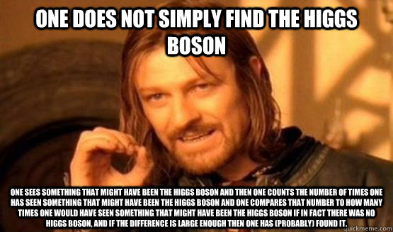
But more often we want to measure something. This is true even for things like the Higgs search, where the initial announcement of the Higgs boson discovery was for “a new particle with a mass between \(125\) and \(127\) \(\text{GeV}/c^2\)”. It’s even more true in other contexts. In medicine, we want to know how effective a drug will be; in psychology we want to know how strongly a picture can affect our emotions; in public policy we want to know how much a new program will reduce poverty.
And neither Fisher nor Neyman-Pearson answer those questions at all. It’s just not what they’re designed to do.
I talked about this problem in my post on the replication crisis. Amy Cuddy started by asking whether the power pose had an effect—a yes-or-no question. She wound up talking about how large the effect was, which is a completely different question. Hypothesis testing only answers the first question; if you try to use it to measure things you cause yourself all sorts of problems, just like the ones Cuddy ran into.
We also see these problems in research on politically controversial subjects like the minimum wage and gun control. Economic theory suggests that raising the minimum wage should increase unemployment; there’s an extensive literature of dueling empirical studies, with some showing that it does, and others showing that it doesn’t. A lot of ink has been spilled over whether minimum wage increases really increase unemployment, and that’s a genuinely tricky question that I can’t answer.11
But what I can do is reframe the question. We don’t know if the minimum wage raises are increasing unemployment. But we do know they can’t be increasing it very much. If they were, we’d be able to tell! So the effect may be real, but if it is, it’s small.12 That’s a good enough answer to make policy. But it’s not an answer that hypothesis testing can give you.
If we care about the size of what we’re studying, and not just whether it exists at all, there are much better tools to use than hypothesis tests like Fisher or Neyman-Pearson. I’ll talk about some of these in Part 3 of this series.
The Significance Binary
The other major difference between Fisher’s approach and Neyman-Pearson is the degree of nuance allowed in their answers. In Fisher’s formulation, we ask how much evidence our experiment gives against the null hypothesis, which means we can have a lot of shades of gray in our result. The lower the \(p\)-value, the stronger the evidence; a \(p\)-value of \(0.001\) is ten times as good as a \(p\)-value of \(0.01\).
This still doesn’t measure the size of the effect, because you can have lots of evidence for a small effect. (I have plenty of evidence that I can move things by pushing them with my finger, but that won’t allow me to knock over the Washington Monument.) But Fisher’s methods do give a fine-grained, quantitative measurement of something: the strength of the evidence against our null hypothesis.
In contrast, the Neyman-Pearson formulation doesn’t give us fine distinctions. We ask if our alternative hypothesis is better than the null, and we get an answer to exactly that question—and that answer can only be “yes” or “no”. The entire continuous \(p\)-value spectrum gets compressed into a definitive “yes” or “no” with no middle ground.
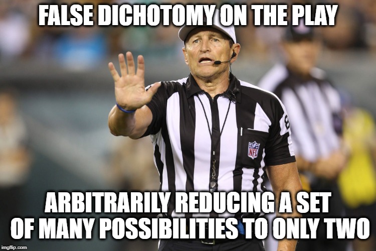
That’s a huge problem when nuance is important, with consequences visible throughout the body of scientific literature. But the problems especially bad in contexts like public health communication, where both honesty and clarity save lives.
Our medical establishment uses what’s essentially a Neyman-Pearson framework to evaluate possible treatments. And it is (understandably) conservative about approving new drugs, which means that \(\alpha\) is set fairly aggressively. We get a lot of false negative results, denying treatments that would work. And in a terrible misuse of language, when a treatment doesn’t clear our fairly high bar for significance, we tend to say there is “no evidence” for it, or even flatly that it “doesn’t work”—whether we mean that it definitely doesn’t work, or that it probably does but we’re not quite sure yet.
This failing was on full display in the early days of the coronavirus pandemic. In February and March 2020, the Surgeon General issued a statement that masks “are NOT effective in preventing” Covid infections, even though we had good reasons to believe they were; the evidence was real, but not (yet) sufficient to reject the null. In December, the World Health Organization said there was no evidence that vaccines would reduce covid transmission. Again, there was real evidence that vaccines would reduce transmission, but not enough to cross WHO’s Neyman-Pearson-style decision threshold. And because of the binary output of a Neyman-Pearson process, this tentative wait-and-see approach was communicated in the form of definitive, final-sounding judgments.
There are definitely smarter and more sophisticated ways to use hypothesis testing on questions like this. First, it would help just to remember that our results are provisional and not absolute truths. Sometimes we do have to make a decision now about whether to prescribe a treatment, or roll out a new product, or even just change some official guidelines. But that doesn’t mean we’re locked into that decision forever; and simply saying there was “not enough” evidence for masks, rather than “no evidence”, would have been more honest and also made the subsequent reversal less confusing.
Second, when we do have to make decisions, we can be more thoughtful about the trade-offs between false positives and false negatives. It’s become standard to take \(\alpha=0.05\) and let \(\beta\) fall where it may; but the decision theory works best when we think about the actual trade-offs involved, and choose our parameters accordingly. That, too, would have helped with communication around Covid: the risks of having people wear masks for a couple months while we figured out if they helped were low, and we didn’t need to be as cautious about recommending masking as we are about approving a new cancer drug.
Where do we stand?
Hypothesis tests are ways of using data to give yes-or-no answer to certain questions. They’re extremely powerful in the contexts they were designed for: Neyman-Pearson gives a good rule for making decisions, and Fisher gives a good approach to describing how much evidence your experiment produced. But when you try to apply them outside of those contexts, you can easily get confusing or misleading results.
But this essay has presented both approaches to hypothesis testing more or less as they were originally designed, in their original contexts. Modern hypothesis testing works a little differently. The Fisher approach gives us a nuanced evaluation of the evidence, but no firm conclusion; the Neyman-Pearson approach gives us a clear answer, but nothing else.
But modern researchers often want both. Modern methods try to deliver. And modern methods often, predictably, fail.
Next time in Part 2 we’ll see how the modern approach to hypothesis testing works. And we’ll see how the modifications we’ve made to try to have it both ways loses some of the benefits of both approaches, and invites the sort of research failures that we’ve seen throughout the replication crisis.

Have questions about hypothesis testing? Is there something I didn’t cover, or even got completely wrong? Or is there something you’d like to hear more about in the rest of this series? Tweet me @ProfJayDaigle or leave a comment below.
-
Some of these specific people were pretty awful in one way or another. Ronald Fisher in particular was racist and a vigorous defender of tobacco companies, though Jezry Neyman seems to have been perfectly lovely. I’m not going to go into detail about their failings, among other things because I’m not especially well-informed on the subject; I recommend the articles I linked if you want to know more. ↵Return to Post
-
Much of this essay, and especially the historical information on the way these schools of thought developed, draws heavily on the article Confusion Over Measures of Evidence (\(p\)’s) Versus Errors (\(\alpha\)’s) in Classical Statistical Testing by Hubbard and Bayarri. This extremely readable article is also a fascinating historical artifact, basically predicting the entire contour of the replication crisis in 2003. ↵Return to Post
-
Okay, maybe I didn’t actually expect my car to be accurate and unbiased. But it’s at least supposed to be true, so it provides a good baseline for comparison. ↵Return to Post
-
You might worry about whether it’s a two-sided but biased coin. But Gelman and Nolan have argued that coins physically can’t be biased, and I find their argument compelling. If you don’t find it compelling, you have to decide how likely you think a weighted coin would be—which is exactly the “other evidence” that Fisher’s paradigm doesn’t even try to account for. ↵Return to Post
-
A friend asks if meta-analysis accomplishes the same thing, but meta-analysis is actually a much weaker threshold than the one Fisher gives here. Meta-analysis tries to amplify weak signals and reconcile inconsistent results; Fisher says we should only believe a claim when we can consistently get a strong signal. ↵Return to Post
-
From what I understand, Fisher was a little contemptuous of the idea that you could answer this question mathematically. ↵Return to Post
-
I’m not convinced I agree with this, but that’s beside the point here. I’ll discuss this choice a bit more in Part 2 of this series. ↵Return to Post
-
In a medical context, we often talk about the related concepts of sensitivity and specificity. Sensitivity is the “true positive” rate \(1-\beta\), the probability of correctly prescribing the drug if it would help. Specificity is the “true negative” rate \(1-\alpha\), the probability of correctly withholding the drug if it would not help.
These terms come from diagnostic testing. “Sensitivity” measures the chance of correctly detecting a condition that you have; “specificity” measures the chance of correctly detecting that you don’t have a condition. ↵Return to Post
-
All three were frequentists, and believed (roughly) that you can only give a “probability” for something repeatable. You can talk about the probability a study will give a null result, since you could run a hundred studies and count how many give the null. But you can’t talk about the probability that a given drug works, since there’s only the one drug.
The major modern alternative to frequentist probability is Bayesianism, which does think this question makes sense. I’ve written about Bayesian reasoning [in the past] and I’ll come back to it in Part 3 of this series. But the Neyman-Pearson method is definitely not Bayesian. ↵Return to Post
-
Modern researchers have ways to get around that using tools like meta-analysis: at any given time you can make a decision based on all your information, and when you get new information you can make a new decision. But it’s still a bit forced, and not what Neyman-Pearson was designed for. ↵Return to Post
-
Among other things, because the answer is probably “sometimes yes and sometimes no, it depends on the circumstances.” And I don’t think anyone seriously doubts that a minimum wage of \$100 per hour would increase unemployment, and a minimum wage of \$1 per hour would not. ↵Return to Post
-
This is the difference between “practical significance” and “statistical significance” we talked about earlier. But that distinction shouldn’t arise in a proper Neyman-Pearson setup, which is one way you can tell it’s being misused here. ↵Return to Post
Tags: philosophy of math science replication crisis statistics
 Support my writing at Ko-Fi